How to Create a Makeshift Content Calendar in Excel

How to Create a Content Calendar in Excel

Monitoring your last share date is actually easy to accomplish in Excel or other comparable spreadsheet programs.

You'll need to create four column titles in Row #1 which we recommend labeling Post Title, Last Share Date, Days Since, and Link in cells A1 through D1 respectively. If you want to have an extra row, Comments could be a good one where you can make notes on items like how the last share did, if the content is seasonal and should be shared by a certain date, etc.

From here, each row will represent an individual article. The Post Title and Link columns should feature exactly that- write a title that you'll easily recognize in the respective title box and put the URL hyperlink in the respective link box.

For the Last Share Date, keep this box blank for the time being as these will be manually entered as you share. Whenever you share an article, simply go into this cell and type in the share date in the format of MM/DD/YYYY or, if you are located elsewhere that uses another format, variants like DD/MM/YYYY- either format should work as long as it has day, month, and year.

• For new articles or those we do not know the last share, we sometimes put in 01/01/2000 as a placeholder instead of leaving it blank. We'll discuss why a bit more later.

In the first Days Since cell (C2), you'll want to type the following equation:

=IF(B2=””,””,TODAY()-B2)

Warning: If you copy and paste the above equation into Excel, you may get an error as the quotes are not in the same format that Excel uses for equations (I guess Excel doesn't like our font). If you delete the two quote sets (“”) and retype them manually it should fix this.

This calculation uses an If statement and displays a number result based on the following logic:

• If the Last Share Date in cell B2 is blank, show a blank box here.
• Otherwise, if the Last Share Date box includes is a date, show the difference between today's date and the Last Share Date.
  • The numbers should be positive if the last share was in the past, but this also works for advanced scheduling and will show a negative if a post is scheduled for the future.
  • E.g. a positive 3 means the post was shared three days ago whereas a -3 means the post is scheduled for three days in the future.

If for whatever reason you receive any other errors with the above calculation, an alternative option to try could be the following:

=DAYS(TODAY(),B2)

This one simply brings back the difference between the original date and today's date. But instead of showing an empty cell if B2 is blank (as the above If statement does), it will show a really large number. The reason for this is that Excel seems to start its date calculations on January 1, 1900. So if the last share date is undefined it will use this number as a reference (which at the time of publishing was roughly 44,240 days ago). Just keep that in mind!

In either case, you'll need to ensure that this calculation is in every cell in the C column if the corresponding cells in any given row have data. This can be accomplished by highlighting the cell you first placed the code into (likely C2). When you do this, a small square should be visible in the bottom right corner. Grab that and drag it down to highlight all the boxes in column C that coincide with the filled cells in your sheet. When you let go, this equation should populate all the cells while automatically changing the cell references accordingly (B2 becomes B3 in row three, B4 in row 4, and so on).

• Reminder: If the Last Share Date is blank, the cells here will also display a blank by design if you are using the first equation. You'll have to click on the cell manually to double-check that the equation is there. It should update automatically once a Last Share Date is added.

The neat thing about this is that every time Excel is modified, in any cell, these equations should update automatically (there is a way to turn this feature off in Excel, but I believe it should be on as a default). So if you come back to your file tomorrow, that 0 should automatically update to a 1 and so on. Neat, right?

One of the reasons we put 01/01/2000 as a placeholder for new and/or articles with unknown last share dates is that, as of the time we published this article, it has been over 7,000 days since then. So column C for Days Since should display a stupidly high number (> 7,000) here whereas articles that have been shared may have dates of 1, 10, or 100 days- much smaller by comparison.

The last step here is to simply highlight all your data (click the A column and then hold the shift key and click the D column to highlight all the data below it) and then apply a filter. This can be achieved on the Data tab with the sub-button Filter directly in Excel.

When you do this, arrows pointing down will appear in Row #1 (which should be your labels). Click the down arrow next to Days Since and click the option “Sort Largest to Smallest”. Now all your articles will be organized by the highest Days Since to the lowest and you can easily see what articles haven't been shared in a few weeks, months, or even years.

Easy! And, perhaps even better, those unshared posts that have a date of > 7,000 will always be at the top- a great reminder that they still need to be shared.

It is worth noting that unlike the Days Since calculation, which updates automatically, the sort function is a manual action. The rest of the data will update accordingly as you use this sheet, but you'll want to periodically re-sort to push the older articles back to the bottom. We do this every week or so but your mileage may vary based on how frequently you share content.

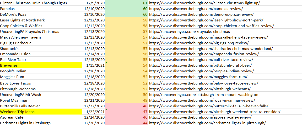
As an added layer, you may also want to play around with the Conditional Formatting rules in the Days Since column to color-code the boxes for articles to help give a visual cue as well. We color code anything green that has been shared > 60 days (ready to share again), yellow 30-60 days (possibly can share again), and red < 30 days (wait to share). This is a great visual cue in addition to the numbers, and updates automatically as well.

Once your sheet is built, there are really only three things you need to do to manage it over time:

• Add new links as articles are published.
• Change the Last Share Date for existing articles whenever you share it.
• Sort the Days Since column periodically to re-organize your articles.

We primarily use this for Facebook shares of articles, but we also have a similar setup for image shares on Facebook as well. You can repeat this process as you like for any social network you regularly share to and it really helps you keep your content calendar streamlined!

So, there you have it, our quick way for creating a content calendar to re-share evergreen content on our social media channels.

How do you go about organizing a content calendar? Do you use a process like the above or something different? Comment below to share your steps!